여러 이벤트의 발생 확률에 대한 확률분포, Dirichlet distribution
1. Intro
한 이벤트가 발생할 확률에 대한 확률 분포를 뜻하는 Beta distribution을 여러 이벤트에 대해 확장한 것이 Dirichlet distribution이다. 기상청에서 ‘화창한 날씨’를 예보하는 상황을 들어보자. 만약 Beta distribution을 사용한다고 하면 이 확률분포는 ‘화창한 날씨’일 확률, 그리고 ‘화창하지 않을 날씨’일 확률에 대한 것일 것이다. ($Pr(‘sunny’)+Pr(‘!sunny’)=1$)
그러나 Dirichlet distribution을 사용한다면 더 많은 이벤트에 대해서 확률 분포를 모델링 할 수 있다. 만약 이벤트를 ‘sunny’, ‘cloudy’, ‘rainy’ 로 구분한다면, ($Pr(‘sunny’)+Pr(‘cloudy’)+Pr(‘rainy’)=1$) 각각의 이벤트가 발생할 확률에 대한 확률 분포가 dirichlet distribution으로 나타나는 것이다.
즉, 다시 말해보자면 위 예시에 대해서 각 이벤트가 발생할 확률을 n개의 확률변수 $x_k(k=1,\cdots,n)$ 로 나타낸다고 하면, Beta distribution의 경우 $n=2$ 로 $x_1+x_2 = 1$ 인 직선을 정의역으로 가지는 확률 분포가 그려질 것이고, Dirichlet distribution의 경우 $n=3$ 으로 $x_1+x_2+x_3 = 1$ 을 만족하는 평면을 정의역으로 가지는 확률 분포가 그려질 것이다.
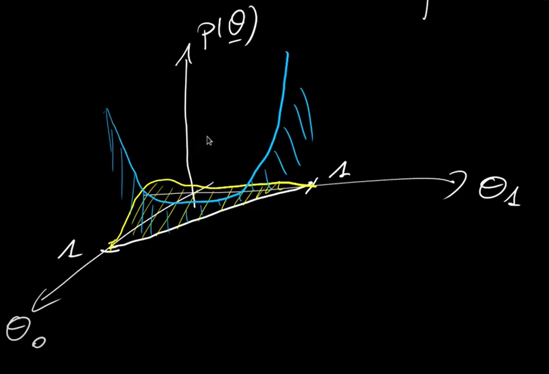 이벤트가 2개인 경우 정의역이 직선으로 나타나는 dirichlet distribution
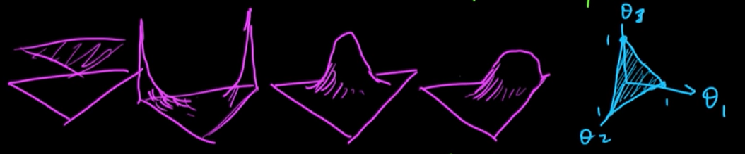 이벤트가 3개인 경우 정의역이 평면으로 나타나는 dirichlet distribution
만약 ‘눈보라’ 라는 이벤트를 추가해서 확률변수가 4차원이면 어떨까? 뭐 별다른 거 없이 $x_1+x_2+x_3+x_4 = 1$ 을 만족하는 정의역에서 dirichlet distribution이 정의될 것이다. 하지만 4차원부터는 시각화를 할 수가 없다. 이벤트가 2차원인 경우 직선, 3차원인 경우 평면이었지만 4차원 이상부터는 이제 부를 호칭이 애매해진다. 그래서 n 차원에 대해서 ‘(n-1)-simplex’로 통일해서 부른다. 그러니까 위 그림에서 삼각형으로 나타나는 평면은 3차원의 2-simplex이고, 직선은 2차원의 1-simplex이다. 참고로 4차원에서 3-simplex는 정사면체이다.
2. Probability density function
Dirichelt distribution의 density function은 beta distribution에서 확률 변수의 차원만 늘어난 것으로, 크게 어려운 형태가 아니다. 예를 들어 3차원 확률변수($\theta_0+\theta_1+\theta_2=1$)에 대하여 경우 각 확률 변수가 나타나는 빈도를 상징하는 $\alpha_0,\alpha_1,\alpha_2$ 가 parameter로 주어진다면, beta distribution의 형태와 비슷한 다음의 식에 비례하는 형태가 될 것이다.
\[\begin{aligned} p(\Theta)\sim\theta^{\alpha_0-1}_0\theta^{\alpha_1-1}_1\theta^{\alpha_2-1}_2,\quad where\:\alpha_0,\alpha_1,\alpha_2>0 \end{aligned}\]이를 D-dimensional 로 일반적인 상황에 대하여 확장하면, 즉, $\Theta\in\mathbb{R}^D$ 인 경우, $\Theta$는 $D-1$ 차원 상의 simplex에 정의되어 있다. 이 simplex의 n-1개의 꼭지점(vertex)는 아래와 같을 것이다.
\[\begin{aligned} \begin{bmatrix} 1 \\\ 0 \\\ \vdots \\\ 0 \end{bmatrix} \begin{bmatrix} 0 \\\ 1 \\\ \vdots \\\ 0 \end{bmatrix} \cdots \begin{bmatrix} 0 \\\ 0 \\\ \vdots \\\ 1 \end{bmatrix} \end{aligned}\]이때 pdf는 다음에 비례한다.
\[\begin{aligned} p(\Theta)\sim\prod_{d=0}^{D-1}\theta_d^{\alpha_d-1} \end{aligned}\]이를 normalize 시키면 최종적으로 다음의 식을 얻을 수 있다.
\[\begin{aligned} p(\Theta)=\frac{\Gamma{(\sum_{d=0}^{D-1}\alpha_d)}}{\prod_{d=0}^{D-1}\Gamma{(\alpha_d)}}\cdot\prod_{d=0}^{D-1}\theta_d^{\alpha_d-1}:=Dir(\Theta,\alpha),\quad where\:\mathbf{\alpha}>\mathbf{0} \end{aligned}\]


Leave a comment